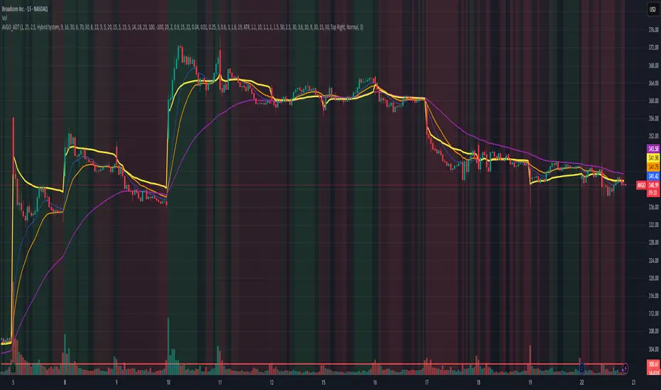
AVGO Advanced Day Trading Strategy📈 Overview
The AVGO Advanced Day Trading Strategy is a comprehensive, multi-timeframe trading system designed for active day traders seeking consistent performance with robust risk management. Originally optimized for AVGO (Broadcom), this strategy adapts well to other liquid stocks and can be customized for various trading styles.
🎯 Key Features
Multiple Entry Methods
EMA Crossover: Classic trend-following signals using fast (9) and medium (16) EMAs
MACD + RSI Confluence: Momentum-based entries combining MACD crossovers with RSI positioning
Price Momentum: Consecutive price action patterns with EMA and RSI confirmation
Hybrid System: Advanced multi-trigger approach combining all methodologies
Advanced Technical Arsenal
When enabled, the strategy analyzes 8+ additional indicators for confluence:
Volume Price Trend (VPT): Measures volume-weighted price momentum
On-Balance Volume (OBV): Tracks cumulative volume flow
Accumulation/Distribution Line: Identifies institutional money flow
Williams %R: Momentum oscillator for entry timing
Rate of Change Suite: Multi-timeframe momentum analysis (5, 14, 18 periods)
Commodity Channel Index (CCI): Cyclical turning points
Average Directional Index (ADX): Trend strength measurement
Parabolic SAR: Dynamic support/resistance levels
🛡️ Risk Management System
Position Sizing
Risk-based position sizing (default 1% per trade)
Maximum position limits (default 25% of equity)
Daily loss limits with automatic position closure
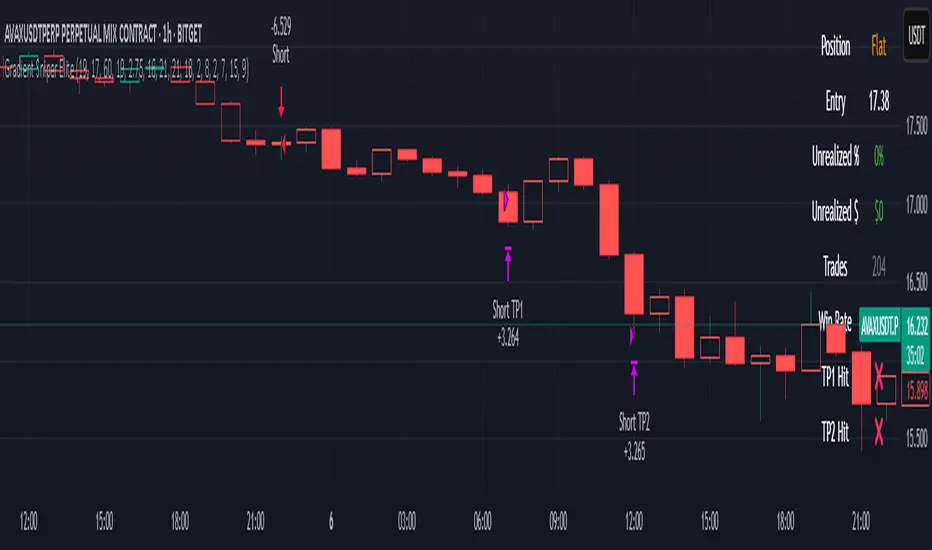
Multiple Profit Targets
Target 1: 1.5% gain (50% position exit)
Target 2: 2.5% gain (30% position exit)
Target 3: 3.6% gain (20% position exit)
Configurable exit percentages and target levels
Stop Loss Protection
ATR-based or percentage-based stop losses
Optional trailing stops
Dynamic stop adjustment based on market volatility
📊 Technical Specifications
Primary Indicators
EMAs: 9 (Fast), 16 (Medium), 50 (Long)
VWAP: Volume-weighted average price filter
RSI: 6-period momentum oscillator
MACD: 8/13/5 configuration for faster signals
Volume Confirmation
Volume filter requiring 1.6x average volume
19-period volume moving average baseline
Optional volume confirmation bypass
Market Structure Analysis
Bollinger Bands (20-period, 2.0 multiplier)
Squeeze detection for breakout opportunities
Fractal and pivot point analysis
⏰ Trading Hours & Filters
Time Management
Configurable trading hours (default: 9:30 AM - 3:30 PM EST)
Weekend and holiday filtering
Session-based trade management
Market Condition Filters
Trend alignment requirements
VWAP positioning filters
Volatility-based entry conditions
📱 Visual Features
Information Dashboard
Real-time display of:
Current entry method and signals
Bullish/bearish signal counts
RSI and MACD status
Trend direction and strength
Position status and P&L
Volume and time filter status
Chart Visualization
EMA plots with customizable colors
Entry signal markers
Target and stop level lines
Background color coding for trends
Optional Bollinger Bands and SAR display
🔔 Alert System
Entry Alerts
Customizable alerts for long and short entries
Method-specific alert messages
Signal confluence notifications
Advanced Alerts
Strong confluence threshold alerts
Custom alert messages with signal counts
Risk management alerts
⚙️ Customization Options
Strategy Parameters
Enable/disable long or short trades
Adjustable risk parameters
Multiple entry method selection
Advanced indicator on/off toggle
Visual Customization
Color schemes for all indicators
Dashboard position and size options
Show/hide various chart elements
Background color preferences
📋 Default Settings
Initial Capital: $100,000
Commission: 0.1%
Default Position Size: 10% of equity
Risk Per Trade: 1.0%
RSI Length: 6 periods
MACD: 8/13/5 configuration
Stop Loss: 1.1% or ATR-based
🎯 Best Use Cases
Day Trading: Designed for intraday opportunities
Swing Trading: Adaptable for longer-term positions
Momentum Trading: Excellent for trending markets
Risk-Conscious Trading: Built-in risk management protocols
⚠️ Important Notes
Paper Trading Recommended: Test thoroughly before live trading
Market Conditions: Performance varies with market volatility
Customization: Adjust parameters based on your risk tolerance
Educational Purpose: Use as a learning tool and customize for your needs
🏆 Performance Features
Detailed performance metrics
Trade-by-trade analysis capability
Customizable risk/reward ratios
Comprehensive backtesting support
This strategy is for educational purposes. Past performance does not guarantee future results. Always practice proper risk management and consider your financial situation before trading.
Strategia Pine Script®